Application to flight data • graphicalExtremes

1 The dataset

library(graphicalExtremes)
library(ggplot2)
library(igraph)

The flights dataset contains daily total delays of major U.S. airlines. For details, see the corresponding documentation page. Below, we plot all airports in the dataset.

plotFlights(plotConnections = FALSE, map = "world", xyRatio = 2)

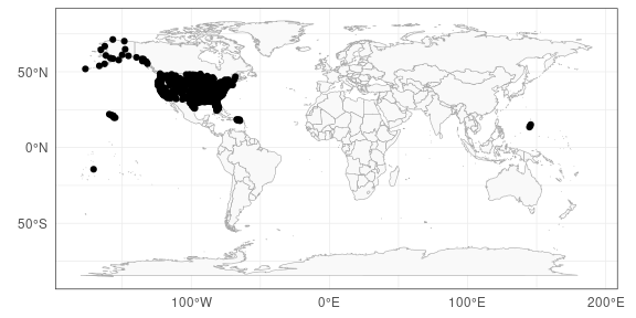
To perform an example application, we follow Section 6 of Hentschel et al. (2022). The subset of airports analyzed there is obtained through a previous clustering step, whose results are available through the function getFlightDelayData(). For more detailed explanations of the individual methods see Vignette “applicationDanube” and the help pages of applied functions. Note: Due to size restrictions, the CRAN version of this package contains only a part of the full dataset. A version of this package with the complete dataset is available on GitHub.

# Get IATAs from Texas cluster
IATAs <- getFlightDelayData('IATAs', 'tcCluster')

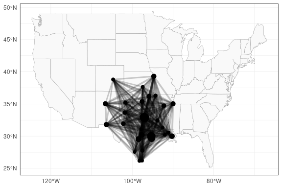
# Plot airports + connections (indicating number of flights by thickness)
plotFlights(
    IATAs,
    useAirportNFlights = TRUE,
    useConnectionNFlights = TRUE
)

For hyperparameter tuning and model comparison purposes, we will use a train-test-split, utilizing some data to estimate the graph structure and parameter matrix, and the remaining data to compute a likelihood value.

# Check whether all dates from the train-test-split are available
# (due to size restrictions, the CRAN version of this package does not contain all dates)
allDatesAvailable <- tryCatch({
    getFlightDelayData('dates', dateFilter = c('tcAll'))
    TRUE
}, error = function(...) FALSE)
cat('All dates avilable:', allDatesAvailable, '\n')
#> All dates avilable: TRUE

# Create train and test data sets
if(allDatesAvailable){
    # Use train-test-split and threshold p from article
    matEst <- drop(getFlightDelayData('delays', 'tcCluster', 'tcTrain'))
    matVal <- drop(getFlightDelayData('delays', 'tcCluster', 'tcTest'))
    p <- 0.95
} else {
    # Take all available dates that do not contain NAs
    mat <- drop(getFlightDelayData('delays', 'tcCluster', 'all'))
    rowHasNA <- apply(is.na(mat), 1, any)
    mat <- mat[!rowHasNA, ]
    
    # Split dates in half
    splitInd <- floor(nrow(mat)/2)
    matEst <- mat[1:splitInd,]
    matVal <- mat[(splitInd+1):nrow(mat),]
    
    # Use a lower threshold to compensate for the smaller dataset
    p <- 0.8
}

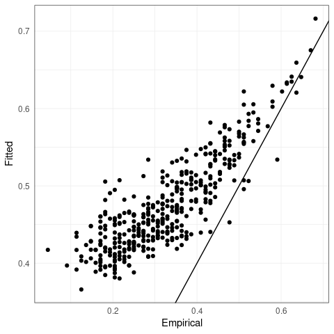
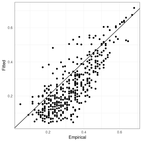
This function will be used later to compare fitted parameters to empirical ones.

# Compute the empirical extremal correlation matrix
emp_chi_mat <- emp_chi(matEst, p = p)

# Utility function to plot fitted parameters against true/empirical ones
plot_fitted_params <- function(G0, G1, xlab = 'Empirical', ylab = 'Fitted'){
    return(
        ggplot()
        + geom_point(aes(
            x = G0[upper.tri(G0)],
            y = G1[upper.tri(G1)]
        ))
        + geom_abline(slope = 1, intercept = 0)
        + xlab(xlab)
        + ylab(ylab)
    )
}

2 Fitting a model to the flight graph

As a baseline for graphical modelling, we consider the graph with edges representing at least monthly connections between airports.

# Compute undirected flights per connection between selected airports
nYears <- dim(flights$flightCounts)[3]
flightsPerConnection <- apply(flights$flightCounts[IATAs,IATAs,], c(1, 2), sum)
flightsPerConnectionUD <- flightsPerConnection + t(flightsPerConnection)

# Make flight graph from adjacency matrix
A <- 1 * (flightsPerConnectionUD > nYears * 12)
flight_graph <- graph_from_adjacency_matrix(A, diag = FALSE, mode = "undirected")

# Plot flight graph
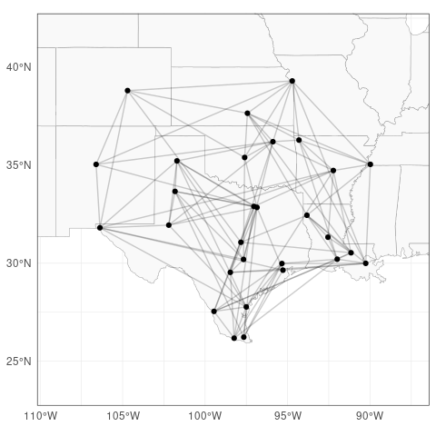
plotFlights(IATAs, graph = flight_graph, clipMap = 1.3, xyRatio = 1)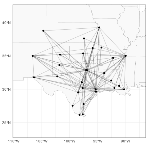

Given the flight_graph object, we fit a Hüsler–Reiss model with that graphical structure.

# Fit the model
model_fit <- fmpareto_graph_HR(
    data = matEst,
    graph = flight_graph,
    p = p,
    method = "vario"
)
#> Error in complete_Gamma(Gamma_partial, graph): Package "edmcr" is required to compute initial completion!

# Compute likelihood/ICs
flights_loglik_graph <- loglik_HR(
    data = matVal,
    p = p,
    graph = flight_graph,
    Gamma = model_fit
)
#> Error: object 'model_fit' not found
cat("Flight graph test-loglikelihood =", round(flights_loglik_graph['loglik'], 2), "\n")
#> Error: object 'flights_loglik_graph' not found

# Plot fitted parameters
plot_fitted_params(emp_chi_mat, Gamma2chi(model_fit))
#> Error in `geom_point()`:
#> ! Problem while computing aesthetics.
#> ℹ Error occurred in the 1st layer.
#> Caused by error:
#> ! object 'model_fit' not found

3 Fitting a tree model

Next, we fit an extremal tree model to the flight delays using emst().

# Fit the model
flights_emst_fit <- emst(data = matEst, p = p, method = "vario")

# Compute likelihood/ICs
flights_loglik_tree <- loglik_HR(
    data = matVal,
    p = p,
    Gamma = flights_emst_fit$Gamma,
    graph = flights_emst_fit$graph
)
cat("Tree test-loglikelihood =", round(flights_loglik_tree['likelihood'], 2), "\n")
#> Tree test-loglikelihood = NA

# Plot fitted graph, parameters
plotFlights(
    IATAs,
    graph = flights_emst_fit$graph,
    xyRatio = 1,
    clipMap = 1.3
)
plot_fitted_params(emp_chi_mat, Gamma2chi(flights_emst_fit$Gamma))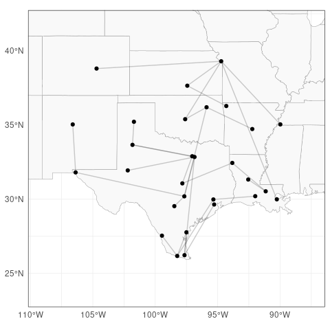

4 Fitting a general model

Lastly, we fit a general graphical model with eglearn(), using a suitable list of penalization parameters.

# Fit the model
rholist <- seq(0, 0.50, length.out = 11)
flights_eglearn_fit <- eglearn(matEst, p = p, rholist = rholist, complete_Gamma = TRUE)

# Compute likelihood/ICs
flights_loglik <- sapply(seq_along(rholist), FUN = function(j) {
    loglik_HR(
        data = matVal,
        p = p,
        Gamma = flights_eglearn_fit$Gamma[[j]],
        graph = flights_eglearn_fit$graph[[j]]
    )
})

The “best” penalization parameter can be chosen e.g. such that the test-likelihood is maximized

ggplot(
    mapping = aes(x = rholist, y = flights_loglik['loglik', ])) +
    geom_line() +
    geom_point(shape = 21, size = 3, stroke = 1, fill = "white") +
    geom_hline(aes(yintercept = flights_loglik_graph['loglik']), lty = "dashed") +
    geom_hline(aes(yintercept = flights_loglik_tree['loglik']), lty = "dotted") +
    xlab("rho") +
    ylab("Log-likelihood") +
    scale_x_continuous(
        breaks = rholist,
        labels = round(rholist, 3),
        sec.axis = sec_axis(
            trans = ~., breaks = rholist,
            labels = sapply(
                flights_eglearn_fit$graph,
                igraph::gsize
            ),
            name = "Number of edges"
        )
)
#> Warning: The `trans` argument of `sec_axis()` is deprecated as of ggplot2 3.5.0.
#> ℹ Please use the `transform` argument instead.
#> This warning is displayed once every 8 hours.
#> Call `lifecycle::last_lifecycle_warnings()` to see where this warning was
#> generated.
#> Error in `geom_hline()`:
#> ! Problem while computing aesthetics.
#> ℹ Error occurred in the 3rd layer.
#> Caused by error:
#> ! object 'flights_loglik_graph' not found

best_index <- which.max(flights_loglik['loglik',])
cat('Best rho =', rholist[best_index], '\n')
#> Best rho = 0.15
cat('Corresponding test-loglikelihood =', flights_loglik['loglik', best_index])
#> Corresponding test-loglikelihood = 1123.673

We plot the estimated graph and parameters of the best fitted model.

best_graph <- flights_eglearn_fit$graph[[best_index]]
best_Gamma <- flights_eglearn_fit$Gamma[[best_index]]
plotFlights(IATAs, graph = best_graph, clipMap = 1.3, xyRatio = 1)
plot_fitted_params(emp_chi_mat, Gamma2chi(best_Gamma))

References

Hentschel, M., Engelke, S., and Segers, J. (2022). Statistical inference for Hüsler-Reiss graphical models through matrix completions. arXiv. https://doi.org/10.48550/ARXIV.2210.14292